Dr. Han Hu: "We developed an Isogeometric analysis numerical framework using a complete variational approach to address nonlinear flexoelectric problems. This framework considers the piezoelectric effect, flexoelectric effect, and Maxwell stress effect of the dielectric. To illustrate its capabilities, we simulated a cantilever beam subjected to a constant torque at the right end, showcasing the direct flexoelectric effect where deformation generates electricity across the beam."


Fig1. Animation of a beam deformed due to electric loading. The colormap indicates the Von-mises stress distribution. Model parameters: thickness H = 1 μm, length L = 20H, Young’s modulus Y = 1GPa, Poisson’s ratio ν = 0.3, dielectric constant ϵ = 0.092 nC/Vm, characteristic length ls = 0, μL = 0 and μT = 10 nC/m, applied electric potential Φ0 = 1.469 kV.


Fig 4. Animation of a beam deformed due to mechanical loading. The colormap indicates the electric potential distribution. Model parameters: thickness H = 1 μm, length L = 20H, Young’s modulus Y = 1GPa, Poisson’s ratio ν = 0.3, dielectric constant ϵ = 0.092 nC/Vm, characteristic length ls = 0, μL = 0 and μT = 10 nC/m, applied moment M0 = 30 Nm.
Fig 5. Schematic of a cantilever beam with open circuit setting.
Additionally, we demonstrated the converse flexoelectric effect by applying a prescribed electric potential to the top surface of the beam, causing significant deformation and warping into a circular shape.
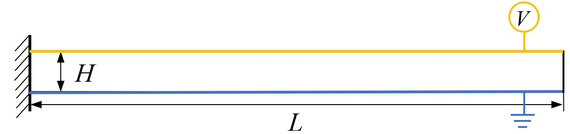
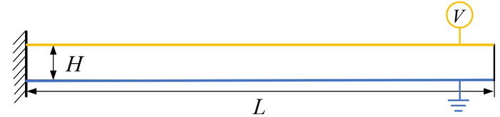
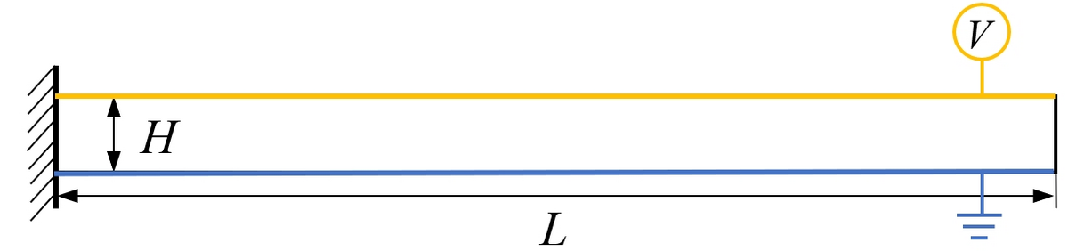
Fig 2. Schematic of a cantilever beam with closed circuit setting.
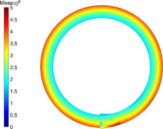


Fig 3. Von-mises stress distribution of the deformed cantilever beam at final configuration.


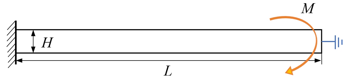
Fig 5. Schematic of a cantilever beam with open circuit setting.

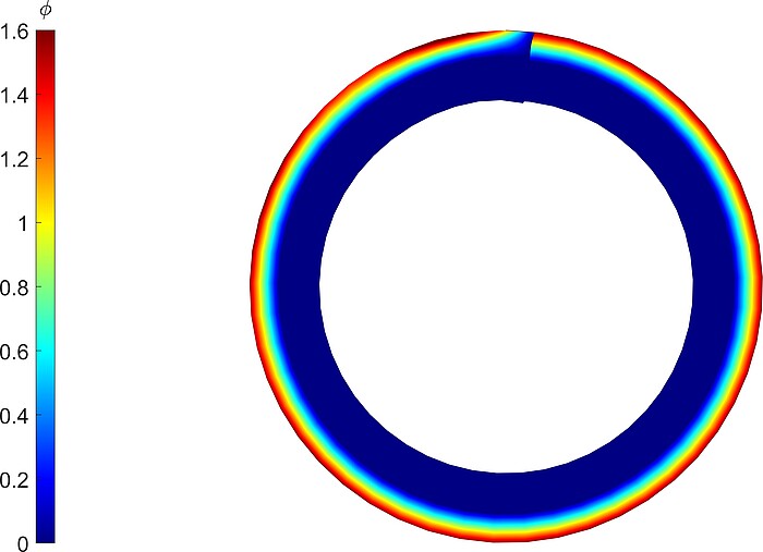

Fig 6. Electric potential distribution of the deformed cantilever beam at final configuration.


